This article is also available as a Jupyter notebook on Google Colab.
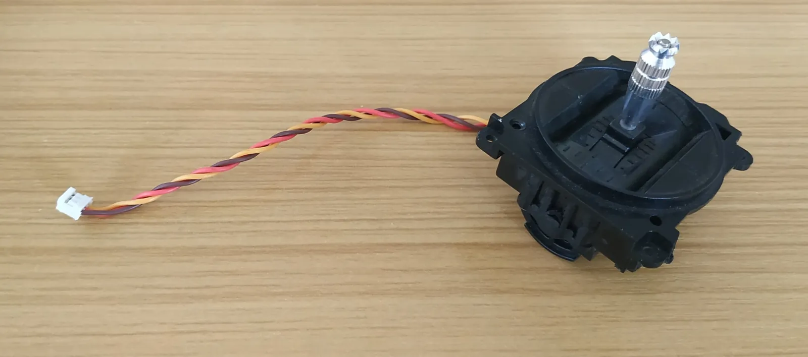
I was upgrading a gimbal in an R/C controller when I noticed that the design of gimbal zeroing mechanism was a relatively non-obvious invention. I’ve seen this zeroing design on gimbals from more than one manufacturer, so I thought I would take a closer look. First, here’s the mechanism in action:
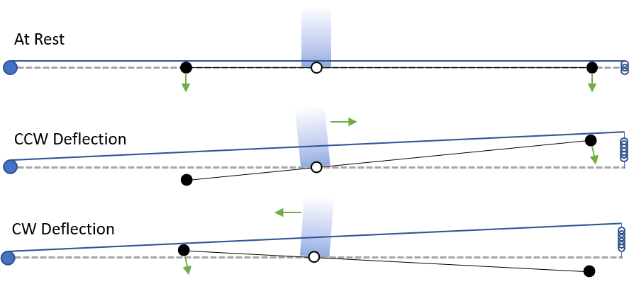
Each axis is has a separate centering mechanism with its own tension spring to provide the inwards force. As the gimbal is pushed away from the center position, the pin carriage it is attached to rotates. One of two pins on the carriage deflects a spring arm, which stretches a spring and provides the restorative force. Here’s a diagram:
The Problem
What we want from such a gimbal design is the restoring force for both positive and negative deflections to be similar. This gimbal is noticeably stiffer when deflected rightwards than leftwards side than the other. This is very annoying during regular use, so lets see if we can fix this.
Simple Model
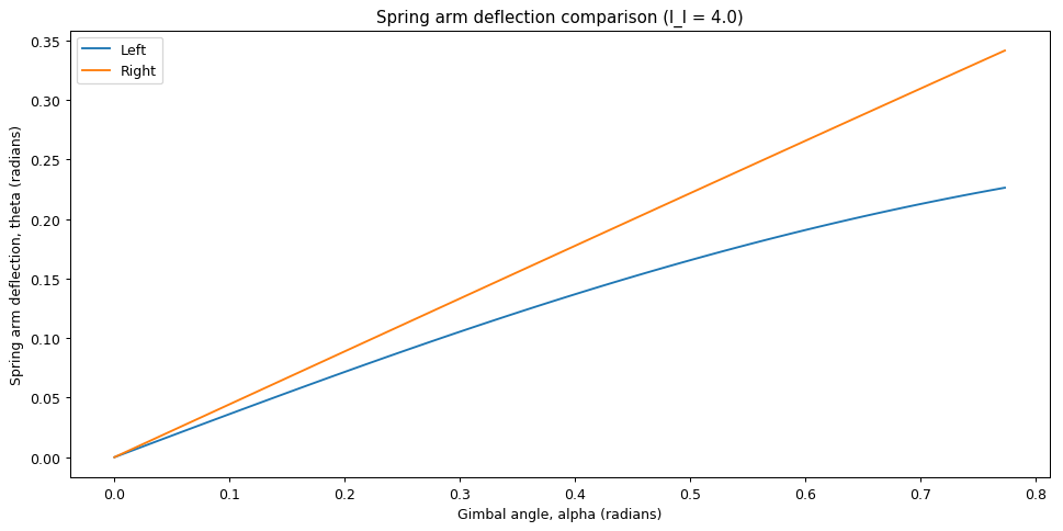
We assume a simple geometry with a frictionless side and a pin of infinitesimal radius. The radius of the gimbal base is \(r = 15 \text{mm}\), and right-side pin is \(l_r = 12 \text{mm}\) from the center. Using some high-school geometry, we can calculate the angle of deflection of the spring arm \(\theta\) as a function of the gimbal angle \(\alpha\):
\[ \theta = \max\left( \tan^{-1}\left(\frac{\sin(\alpha)}{\frac{r}{l_l} - \cos(\alpha)}\right), \tan^{-1}\left(-\frac{\sin(\alpha)}{\frac{r}{l_r} + \cos(\alpha)}\right) \right) \]
Measuring the left-side pin to be about \(l_l = 4mm\) from the center, this looks like:
def theta(alpha : float, radius=None, arm_l=None, arm_r=None):
  theta_l = atan(sin(alpha) / (radius/arm_l - cos(alpha)))
  theta_r = atan(sin(alpha) / (radius/arm_r + cos(alpha)))
  return theta_l, theta_r

def plot_theta(X, theta, radius=None, left_l=None, right_l=None):
    ...

gp = {"radius": 15., "right_l": 12., "left_l": 4.} # Gimbal properties
X = np.arange(0, np.pi/4, np.pi/4/64) # Range
plot_theta(X, theta, **gp)
Now that we have this function, we can find a new left-pin distance \(l_l\) to minimize the difference in the two forces. We do this by constructing a loss function that penalizes the difference between the left- and right-side force at evenly spaced points:
def loss(radius=None, left_l=None, right_l=None):
  X = np.arange(0, np.pi/4, np.pi/4/64)
  return sum(abs(l-r) for l, r in (theta(x, radius, left_l, right_l) for x in X))
# Construct a partial loss function
loss_partial = lambda x: loss(radius=gp["radius"], left_l = x, right_l = gp["right_l"])
We use the Golden Section search from SciPy’s minimize_scalar optimizer to find a minimizing value.
left_l_opt = minimize_scalar(loss_partial, bracket=[1e-5, gp["right_l"]], method="golden")
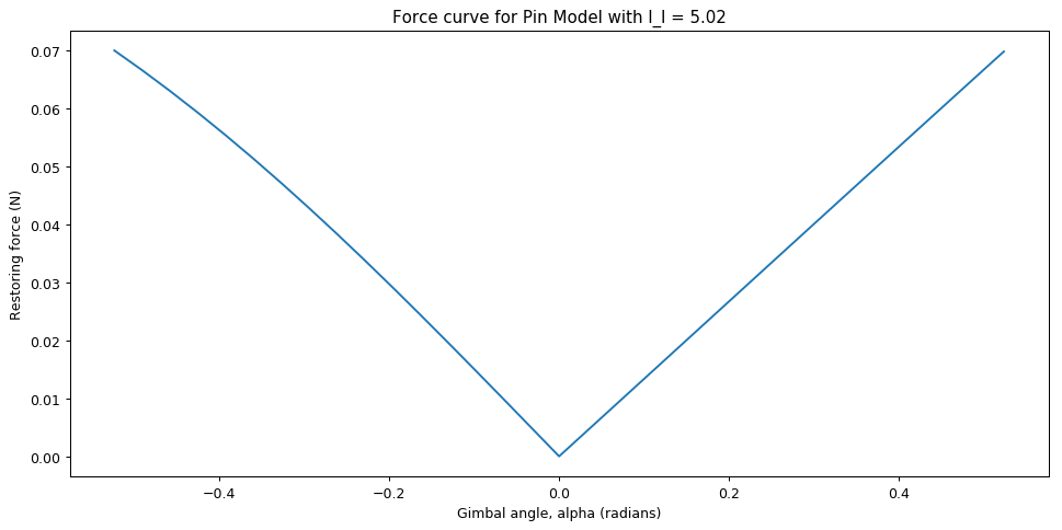
After a few seconds, we get \(l_l = 5.02 \text{mm}\), which produces this curve:
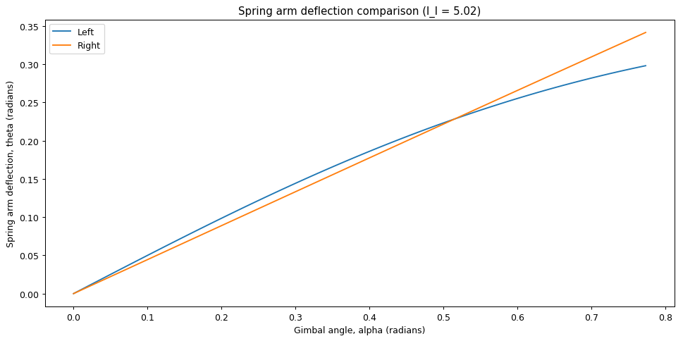
Its much closer, and would be much more difficult to feel in the gimbal movement. Now let’s explicitly model the force-response curve:
Force curves
The output angle is useful to find a value of \(l_l\) that minimizes the difference in response, but ultimately we care about the force-response curve. Consider a preloaded spring (already stretched some distance d) with spring coefficient k=0.01 N/mm. We model the force response curve:
def theta_to_force(theta, d=None, k=0.01, radius=None):
  return max((radius*4*abs(sin(theta/2)) + d), 0) * k

def plot_force(X, radius=None, left_l=None, right_l=None, d=None, k=0.01):
  ...
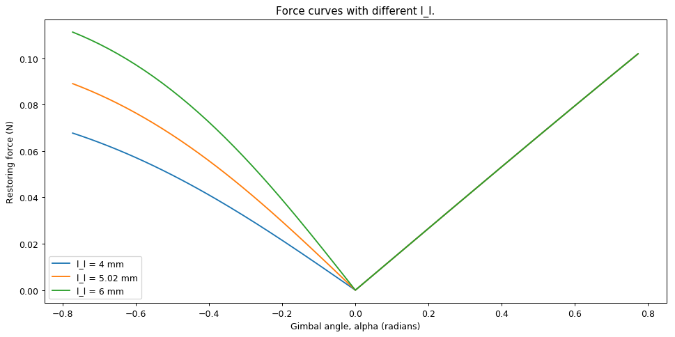
We can compare the force curves for different values of \(l_l\). At our optimal value, the difference between the left and right sides is barely perceptible.
plot_force(..., left_l=4), plot_force(..., left_l=5.02), plot_force(..., left_l=6)
Pin-Diameter Model
So far, so simple. The problem with our model is the diameter of the pins (\(\sim 1 \text{mm}\)) is significant compared to the displacement. This means the point of contact between the spring arm and pin carriage slides along the spring arm as the angle changes.
We model this using sympy, which lets us perform symbolic geometry calculations (among other things). It is overkill for this project, but is an interesting tool to explore.
Sympy behaves a lot like a dataflow system. It allows you to define symbols, which are placeholders for values. You can perform operations (derivatives, translations, rotations, etc.) in terms of these symbols, and ultimately substitute real values and obtain solutions.
We begin by defining the problem in terms of the symbols:
import sympy as sym

# Structure of pins:
r  = sym.symbols("r")  # radius
ll = sym.symbols("ll") # length_left, as a fraction of the radius
lr = sym.symbols("lr") # length_right, as a fraction of the radius
a  = sym.symbols("a")  # alpha
t  = sym.symbols("t")  # theta
pr = sym.symbols("pr") # pin radius
v  = sym.symbols("v")  # vertical displacement of pin arm
We describe the pin carriage in terms of these symbols. It passes through the origin and is rotated by angle a. The left and right pins extend ll/r and lr/r units along the line.
center = sym.Point(0, 0)
pin_arm = sym.Line2D(center, sym.Point(r, 0)).rotate(a)
right_pin = pin_arm.arbitrary_point(lr)
left_pin = pin_arm.rotate(sym.pi).arbitrary_point(ll)
We can check our work with symbolic solutions for these! For example, SymPy evaluates left_pin to Point2D(lr*r*cos(a), lr*r*sin(a)).
Similarly, we construct the spring arm. This is anchored at (-r, v) and is rotated by angle t.
# Point at which the lever is fixed:
lever_fix = sym.Point(-r, v)
lever_arm = sym.Line2D(lever_fix, sym.Point(r, v)).rotate(t, lever_fix)
We assume that the pin is touching the spring arm some distance c/(2r) along the spring arm. We create an additional symbol c and model the contact point as being pin_radius away from c:
# Point where the lever arm touches the pin:
c = sym.symbols("c")
lever_arm_intersection_point = lever_arm.arbitrary_point(c)
pin = sym.Point(pin_radius, 0).rotate(t - sym.pi/2)
lever_arm_contact_point = lever_arm_intersection_point + pin
So far, we have constructed the spring arm and the pin carriage separately, without modeling the contact between the two. We do this by assuming each pin touches the spring arm and calculating the corresponding theta. The binding pin (the pin lifting the spring arm) will have the higher theta.
# A utility function to perform symbol substitution
def subst(e, alpha, radius=15, l_left=5, l_right=12, arm_displacement=1., pin_radius=1., theta=None, c=None):
    ... # Substitute values for symbols.

def solve(*args, **kwargs):
    # Assume left pin is touching the spring arm:
    closest_l = subst(lever_arm_contact_point - left_pin, *args, **kwargs)
    p_closest_l = sym.solve((closest_l.x, closest_l.y), (t, c))
    t_l, _ = select_solution(p_closest_l) # Select a valid solution

    # Assume right pin is touching the spring arm:
    closest_r = subst(lever_arm_contact_point - right_pin, *args, **kwargs)
    p_closest_r = sym.solve((closest_r.x, closest_r.y), (t, c))
    t_r, _ = select_solution(p_closest_r)

    binding = "left" if (t_r > sym.pi) or t_l > t_r else "right"
    return (t_l if binding == "left" else t_r), binding
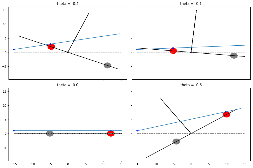
Now that we have a way to model this, we can render images for different gimbal displacements:
Optimizing This
Now that we have a model, we can optimize this exactly as we did before. This takes about half an hour to run on Google Colab:
X_left  = np.arange(-np.pi/6,  1e-4,  np.pi/6/8)
X_right = np.arange( np.pi/6, -1e-4, -np.pi/6/8)
# Precompute right-side deflection:
T_right = [g.get_theta(xr, radius=gp["radius"], l_left=gp["left_l"], l_right=gp["right_l"])[0] for xr in X_right]

def loss(radius=None, left_l=None, right_l=None):
  T_left = [g.get_theta(xl, radius=radius, l_left=left_l, l_right=right_l)[0] for xl in X_left]
  return sum(abs(tl-tr) for tl, tr in zip(T_left, T_right))
loss_partial = lambda x: loss(radius=gp["radius"], left_l = x, right_l = gp["right_l"])
left_l_opt = minimize_scalar(loss_partial, bracket=[1e-5, gp["right_l"]], method="golden")

plot_gimbalsym_theta(...)
The new optimum is at \(l_l = 4.83 \text{mm}\), which produces this response curve:
Great!