On Speculative Decoders

TL;DR: use the model’s own MTP path; most models ship with one. Otherwise, start from the fastest quant and engine, and benchmark the model on your workload at your concurrency. Keep watching this area, new and improved drafters are released often.

These results were benchmarked autonomously by Opus 4.8 and Opus 5 on an NVIDIA DGX Spark, generously provided by Ray Aun Fan.

---

Much of the work on faster inference targets datacenter-scale systems: batching, disaggregation, and enormous KV-cache pools. Speculative decoding is one of the few advances that is also useful for small-scale local inference.

A speculative decoder (also called a draft model, drafter, or speculator) is a small, inexpensive predictor that guesses the next few tokens the large model is likely to produce. The large, or target, model checks those guesses in one pass. In one sweep, it accepts the tokens that match (plus one additional), then resumes normal decoding at the first disagreement.

When the guesses are accurate, one target-model pass can produce 10 or more tokens instead of one. This sounds like a clear win, but there’s a trade-off with the cost of the drafter and verification steps. The rest of this article measures that tradeoff.

Importantly, the choice of next token is always the same as the target. A poor quality drafter can only hurt the speed, not the quality of generation.

How it Works

Speculative decoders propose the next few tokens in a sequence, which can be confirmed in by the target in a single pass.

	prefill	generation
Start	I saw her duck
Draft	I saw her duck	under	the	table	cloth	from the cheap drafter
Verify	I saw her duck	under	the	table	cloth	one target pass all four at once
		✓	✓	✗	—
Resample	I saw her duck	under	the	branch	cloth
reach rate		≈86%	≈71%	≈59%	≈48%

Here’s how this works:

1. Once the prefill is complete, the drafter produces one (or more) possible continuations. This is the draft.

2. In a single verify pass the distribution after each token in each continuation is calculated.

   a. The longest continuation that passes validation is accepted. In the verify row, under the is accepted, table is rejected, and the rest of the draft (cloth) is discarded, however good it looked.

   b. If a token is incorrect, the computed distribution is used to sample a correct one.

   c. If the entire continuation is correct, the computed distribution after the last token is used to sample the “bonus” token.

3. The corrected or bonus token is sampled from the distribution.

   a. For MTP: when the final token is sampled, the next continuation is also computed alongside it.

All four checks happen in that one target pass, so a rejection costs no extra compute; the target resamples branch in the same pass, and decoding continues from there. It is possible to verify the entire sequence in one pass because decode is memory-bound, not compute-bound. There is typically enough compute available to verify even up to 256 possible continuations.

The options

This article considers three families of speculative decoders:

• MTP (multi-token prediction): prediction heads included with the model, or a model-matched assistant checkpoint exposed through the engine’s MTP path. This is usually the lightest option.
• EAGLE3: a separate, small draft head attached to the target model. It reads activations from several layers to make its predictions, and its quality depends heavily on the draft checkpoint.
• DFlash: an external diffusion-based drafter that proposes many tokens per step — up to 16 in these configurations. It has a high fixed cost but can deliver large speedups. DDTree is an extension of DFlash that proposes a tree of continuations rather than a single line.

The results below come from 199 completed benchmark configurations on an NVIDIA DGX Spark, generously provided by Ray Aun Fan — thank you, Ray. An Opus 4.8 (and later, Opus 5) agent ran the benchmarks semi-autonomously. Unless stated otherwise, concurrency is 32.

Five rules of speculation

Speculation pays off only when the system has enough compute available and the acceptance rate is high enough to recover the drafting and verification overhead. This tension is at the core of these five rules:

1. Drafters trade compute for speed
2. Drafters are brittle
3. Agreement is critical
4. Slower target, bigger relative win
5. Speculation can’t fix broken

Rule 1 — Drafters trade compute for speed

As the GPU approaches saturation, the drafter increasingly competes with normal requests for compute.

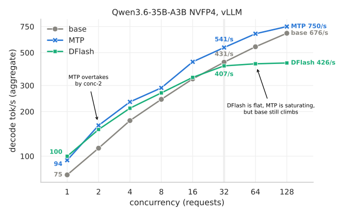
Figure 1 — The concurrency crossover. DFlash narrowly wins at conc-1; MTP overtakes it at conc-2 and reaches 750 tok/s at conc-128. The heavy DFlash drafter beats the no-spec baseline only at low concurrency and slips below it from conc-32 on.

Native MTP drafters are lightweight, so provide a consistent performance boost over the base. As concurrency (and therefore workload) increases the gap narrows but never quite crosses over.

In comparison, external DFlash drafters are much heavier. For this already-fast model, DFlash only narrowly beats the built-in MTP. As concurrency grows, it falls behind MTP and eventually even behing using no drafter at all.

Rule 2 — Drafters are brittle

Drafters are evaluated against the target model’s token choices and often use the target model’s internal state. That makes drafting inexpensive, but also fragile. A plausible token is not enough: the target must assign it an outcome that passes the speculative decoding acceptance rule.

In practice, effectiveness depends on:

1. the drafter model,
2. the exact training and quantization of the target model,
3. the workload, and
4. the serving software.

This extreme sensitivity is because the drafter only helps as much as it produces the same distribution as the target, not just the same tokens. This distribution is changed by quantization, post-training, and even kernel/engine details. Drafter models are small (for speed), and so tend to perform well on narrow workloads. As a separate code pathway, they may also cause scheduler interference or cache weirdness. Here are two examples of this in action:

Swap the engine — Gemma-4-12B with its native MTP head:

engine · quant	base → MTP (tok/s)	Δ
vLLM · NVFP4	504 → 782	+55.0%
SGLang · NVFP4	387 → 400	+3.4%
llama.cpp · Q4	195 → 202	+3.5%

Table 1 — Same drafter, three engines. Gemma-4-12B with its native MTP head, conc-32.

Same model, same drafter, same hardware. Turning MTP on made SGLang switch off its own overlap scheduler, which hides CPU work behind GPU compute — so most of the drafter’s gain went to paying for the scheduling it displaced.

Swap the draft — gpt-oss-120b with EAGLE3:

engine · draft	base → EAGLE3 (tok/s)	Δ
SGLang · LMSYS	140 → 172	+22.0%
vLLM · LMSYS	253 → 247	−2.4%
vLLM · NVIDIA	253 → 139	−45.0%

Table 2 — Same engine, three drafts. gpt-oss-120b with EAGLE3, conc-32.

Holding the model and the engine fixed, the draft weights alone move the result by 43 points — NVIDIA’s throughput-tuned draft accepts about 9% of its tokens, LMSYS/SpecForge about 29%. And the fastest configuration is vLLM without any drafter.

Engine bugs

Drafter code is complex and closely coupled to hardware, making it prone to bugs. In the first few weeks after the launch of a new algorithm expect to see launch errors, missing kernels, unexpected slowdowns, or — in the worst case — silently incorrect output.

We encountered all of these classes of error. The most notable cases were:

• Qwen 3.6 with vLLM + MTP may silently emit malformed tool calls (#35800) or gibberish (#36872).
• Qwen 3.6’s hybrid attention design is incompatible with DFlash and DDTree.
• Gemma-4’s E4B + MTP drafter can’t be run with NVFP4 quantization. No hand-written kernel was available.
• gpt-oss “harmony” channels may be corrupted by EAGLE3, causing gibberish output(#27626).

Across these tests, speculative-decoding support in serving engines remains brittle. Trust a configuration only after testing the exact model, drafter, engine version, hardware, and a representative workload.

Rule 3 — Agreement is critical to performance

The amount of compute saved compared to the decode pass is often calculated as the accept length, which is the number of tokens accepted (including the bonus token) for each decode pass. The accept length without any drafter is 1.

Accept lengths vary substantially across methods and workloads:

• MTP ^{1, 2, 3, 4} generally accepts 2.6–3.0 of 4.
• EAGLE3^{5, 6} manages 2.0–2.4 of 4.
• DFlash² accepts just 2.3–8.0 of 11, and its tree variant DDTree⁷ gets 3.2–10.5 of 16.

That high variance in DFlash and DDTree is worth examining. The same drafter family with the same target (Qwen3-Coder-30B-A3B) performs wildly differently on different datasets:

draft	chat8 accept-len	speed	code9 accept-len	speed
none	1.00	1.0×	1.00	1.0×
DFlash — one line of 16	2.25	0.9×	7.96	2.7×
DDTree — 64-node tree	3.22	1.1×	9.74	2.8×
DDTree — 256-node tree	3.69	0.9×	10.50	2.3×

Table 3 — Same drafter, two workloads. (paper Table 1) Qwen3-Coder-30B-A3B at batch 1, research harness.

Because DFlash and DDTree are heavy drafters, running them at all slows down decode substantially and need to provide enough performance just to get back to the baseline. Despite an acceptance length comparable to MTP on chat tasks, we get no significant speedup.

On code tasks, the heavy drafters pay for themselves by producing impressive accept lengths and corresponding speedups.

Rule 4 — Slower target, bigger relative win

In these measurements, slower target configurations show larger relative gains from speculation. Intuitively, this is because a configuration that is already cheaper per-token leaves less work to amortize.

Sorting the four Qwen3.6 MTP runs from slowest base to fastest produces a monotonic decline in relative gain:

model · quant	base → MTP	Δ
Qwen3.6-27B · FP8	154.7 → 240.9	+56%
Qwen3.6-27B · NVFP4	187.7 → 274.1	+46%
Qwen3.6-35B-A3B · FP8	286.0 → 407.9	+43%
Qwen3.6-35B-A3B · NVFP4	430.8 → 541.3	+26%

Table 4 — Slower base, bigger relative win. Four Qwen3.6 MTP runs at conc-32 on vLLM, sorted slowest base to fastest.

This is a general rule of thumb, not an absolute. Quantization, architecture, kernels, memory pressure, cache friendliness, and scheduler behaviour all affect this trend. The industry is moving in this direction, however, with the largest local models all coming with speculator support.

In the table above, NVFP4 without a speculator (430.8) still out-decodes FP8 with MTP (407.9); this leads us to rule 5:

Rule 5 — Speculation can’t rescue a bad config

A speculative decoder cannot compensate for a slow base configuration. We’ve already seen two such examples of this:

• In Table 2 gpt-oss-120b, SGLang even with EAGLE3 is slower than bare vLLM. This is an example of a bad engine decision not being recoverable despite a good drafter.
• In Table 4 Qwen3.6-35B-A3B, FP8 even with MTP is slower than bare NVFP4. The speedup afforded by using the native NVFP4 hardware beats the good drafter.

In both, the speculative win is real and the configuration around it is what decides the result. Choose the quantization and engine first, then test speculation on that base.

So… what should I do?

The simplest and most reliable solution: Use the model’s own MTP path if available.

Otherwise:

1. Start from the fastest quant and engine. (Rule 4, 5) Trade off hardware support, software bugs, and model performance to get the quickest baseline.

2. Then measure your concurrency. (Rule 1) For local/interactive use, assume c=1!

3. Search HuggingFace for third-party drafters. Industry (RedHat AI, NVIDIA, LMSYS), Labs (DeepSeek, and EAGLE), and scores of hobbyists.

4. Benchmark your model on your workload. (Rule 2, 3)

   a. The drafter performance affects the acceptance rates, which changes if it is worth it.

   b. Periodically check performance. Changing code, harnesses, and data can all cause performance to degrade over time.

None of these rules replaces benchmarking your own model and workload. The results come from one machine, a handful of engines, and two datasets; they will not transfer cleanly to every deployment. Measure decode throughput at the concurrency you actually use, with prompts representative of your traffic, before committing to a speculator.

The field is also moving quickly. Tree-based drafts, diffusion drafters, drafter-assisted prefill, and target models with speculation built into their architecture may all change the recommendation. Treat this article as a snapshot, not a permanent ranking.

Appendix — What comes next

Diffusion-based models

DFlash and DDTree use a diffusion-based drafter that fills a block of future positions in parallel rather than generating them one at a time. This works extremely quickly at low-concurrency generation.

Google carries diffusion into the target model with DiffusionGemma. There is no separate drafter or verification pass: the model generates 256-token blocks by diffusion and refines them iteratively. On the Spark, we measured 116.0 tok/s at batch 1. That lead does not persist as concurrency rises, and its output quality was also significantly below that of its base model.

NVIDIA takes a different route with Nemotron-Labs-TwoTower: it freezes a standard autoregressive model, Nemotron-3-Nano-30B-A3B, and trains a denoiser on top. The authors report retaining 98.7% of benchmark quality while achieving a 2.42× speedup. The same architecture can both verify and speculate, blurring the line between a diffusion target and a drafter.

Two-tower decoding is a promising point between fully autoregressive and fully diffusion-based generation. Its independent results and serving-engine support will be worth watching.

Drafter-assisted prefill

Everything discussed so far accelerates token generation. A drafter may also help with prefill, the stage in which the model processes the prompt before producing its first token.

In drafter-assisted prefill, a small model scans the prompt and identifies the tokens most useful to the target model. The target then processes only that subset. SpecPrefill (ICML 2025) reports up to a ~7.7× improvement in time to first token on a 405B model, potentially using the same drafter for both prefill and decoding.

For long-context, low-concurrency work — a natural use case for the Spark — it is the next technique I would test.

Appendix — the answer is always identical to what the target would produce

Speculation is not an approximation. The accept/resample rule is built so that the tokens the system emits are distributed exactly as the target model alone would have produced them.

The drafter proposes \(x\) following \(q(x)\); the target weighs it against \(p(x)\):

\[ \text{accept } x \text{ with probability } \min\left(1, \frac{p(x)}{q(x)}\right) \]

That draws from the agreement — the mass the two models share:

\[ p_{\text{agr}}(x) = \frac{\min(p(x),\, q(x))}{1 - \beta} \]

On rejection, the target resamples from the residual — where it has more mass than the draft:

\[ p_{\text{res}}(x) = \frac{\max(0,\, p(x) - q(x))}{\beta} \]

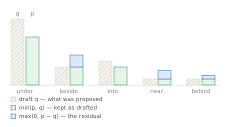
Both normalisers are the same number — the rejection rate:

\[ \beta = 1 - \sum_y \min(q(y),\, p(y)) = \sum_y \max(0,\, p(y) - q(y)) \]

So the weights cancel, and every emitted token is drawn from \(p\):

\[ \Pr[x] = \underset{\text{accepted}}{\underbrace{(1 - \beta)\, p_{\text{agr}}(x)}} + \underset{\text{resampled}}{\underbrace{\beta\, p_{\text{res}}(x)}} = \mathbf{p(x)} \]

In the chart above \(\beta = 0.2\): four times in five the draft token survives, and the one time it does not, the replacement comes from the blue mass the drafter under-weighted. A better drafter shrinks \(\beta\) and so speeds decoding, but it never changes the distribution of the output — only how many target passes it takes to get there.